How to Calulate Gradients Effeciently For ODEs with the Adjoint Method
Often times in engineering and science, we express problems as a system of Ordinary Differential equations (ODEs). Sometimes we are simply interested in how the system evolves over time. However, you might be interested in steering your ODE towards a specific state, such as calibrating your model to real-life data, in which case you need to tune the parameters of your ODE. Is there an efficient way to do this?
Let think of the problem of you trying to hit a target with a ball by adjusting your initial speed and throwing angle. Intuitively, you might throw the ball multiple times to see how the initial speed and angle affects how close you are to the target compared to your initial throw and then adjusting based on the difference. This is basically the finite difference approximation, where you slightly change your model, rerun the model, and record the difference. While, this may work for this problem with only 2 things to worry about, imagine a systems with thousands or hundreds of thousands of possible choices. This is typical for optimisation of FEA models!!. You might then see the issue here. The number of ‘throws’ or solves of our ODE we need to use with finite difference scales with the number of parameters or choices we have and so which can quickly become too unwieldly to use.
However, it turns out there is a method to extract gradients/sensitivities efficiently: the adjoint method. It essentially requires only 2 solves of our ODE system and is independent on the number of parameters in our system circumventing the scaling issue of our finite difference approach.
ODE systems are ubiquitous in all of engineering and science but you might be unfamiliar with them. If you are from an FEA/CAE background, understand that FEA simulations are essentially systems of ODEs. If you are from a machine learning background then you may have heard about the adjoint method in the context of neural ODEs.
The accompanying notebook to this post describes the step by step code for the implementation of the adjoint method outlined by Andrew M. Bradley in this pdf using the ‘simple example’ from the pdf to illustrate the implementation of the adjoint method.The code can be found here.
Because the pdf is concise and therefore dense, it can be quite hard, at a glance, to understand all the points relating to the adjoint method. I recommend looking at the youtube channel Machine Learning & Simulation and his excellent explanation on the adjoint method playlist.
The PDF by Dr. Bradley is more general and applies to Differential Algebraic Equations (DAEs) while the YouTube videos is the adjoint method focused on Explicitely represented ODEs (i.e. can be expressed in the form \(\dfrac{dy}{dt}=f(y,t)\) . For this post we’ll work with the latter type of ODEs
I wrote this notebook to help me learn how the adjoint methods works as well as bridge the gap between these two sources of information. If you wish to understand why each step is performed in the method please look at the links above.
This was written with Python 3.9+ and jax. No GPU is required to run this notebook.
Adjoint Method:
Suppose we have a system that can be represented as a system of explicit ODEs parametised by parameters \(p\) i.e. can be represented in the form
\[\dfrac{dy}{dt} = f(y,t;p)\]That evolves from time \(t=0\) to time \(T\) . Suppose we also have some target object \(F\) (This could be minimisation of cost or distance to a target) that is dependent on some parameters \(p\) If we took the example of trying to aim a trebuchet at a target, \(F\) might be some measure of how close we are to the target while \(p\) might be our intial angle and launch speed.
We want to know how we should best change our parameters to improve our objective. To do so, we need to to calculate \(\dfrac{dF}{dp}\) and then use gradient descent to optimise our objective. To do so we have to calculate the following scary looking equation:
\[\dfrac{dF}{dp} = (\lambda^T\ \partial_{\dot{x}}h)|_{t=0}\ \partial_{x}g^{-1}|_{t=0}\ g_p + \int_0^T (\partial_pf+\lambda^T\partial_ph) \mathrm{d}t\]Using the adjoint method we can solve this using a forward pass (i.e. direct solve) and then the backwards adjoint solve.
- Forward Solve ODE
- Standard solve of inital system of ODEs from \(t=0\) to \(t=T\)
- Backward Solve Adjoint Solution
- Solve the following ODE \(\dot{\lambda} = \partial_xf^T + (\partial_xh)^T\lambda\) from \(t=T\) to \(t=0\)
- Calculate \(\dfrac{dF}{dp}\) using terms calculated from forward and backward pass
- Update parameters via gradient descent ( \(\gamma\) is chosen step size) : \(p_{i+1} = p_i - \gamma \dfrac{dF}{dp}\)
Example
The example we look at, has an analytic solution to check the code at each step. It is from Dr Bradley’s pdf
The Optimisation Problem is as follows:
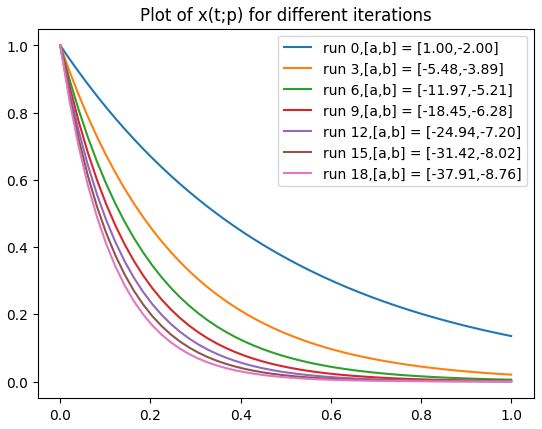
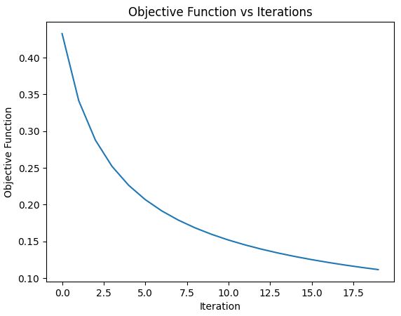
\[\begin{split} \min \int_0^T x \ \mathrm{d}t \\ \mathrm{s.t}\quad \dot{x}= bx \\ x(0) - a =0 \end{split}\]WE can think of this as finding the function x(t) that gives the smallest area given the ODE by changing the parameters a and b
Here the analytical solution of this ODE is : \(x(t) = ae^{bt}\) so our challenge is to find the combination of a and b such that the area under \(x(t) = ae^{bt}\) is minimized.
Note that all stages of this method has an analytical method so you can check the results if you want to try this on your own.
We define the following:
- x : vector of state variables (can also be sometimes called y or u)
- t : independent variable (usually time)
- p : vector representing all parameters
- f : measure of ‘goodness’ such as MSE
- g : is the relationship between the the state and parameters e.g. initial conditions
- h : is the ODE in implicit form
- F : Overall Objective Function across time T
- T : final time So from the problem above we define the following
Our Goal is to find \(\dfrac{dF}{dp}\)i.e. the gradients/sensitivies to change our parameters to improve our objective function.


