Introduction to Physics Informed Neural Networks
Physics informed neural networks or PINNs for short, are a machine learning paradigm where we use neural networks to solve equations that describe physical phenomena such as fluid flow. Physical phenomena are often expressed as a system of differential equations such partial differential equations (PDEs). Typically, we solve these equations using traditional methods such as finite difference, finite element, SPH methods etc. Using PINNs in place of these traditional methods could give us a way to quickly solve and evaluate these equations and open new areas in physics simulations.
Raizzi et al was the first to introduce PINNs in their modern representation. I believe their paper (here) is very approachable to anyone who has done a machine learning course!
This quick tutorial will guide you through the basics of PINNs and the accompanying code in a much simpler example. The code that accompanies this post can be used for extracting arbitrarily high order derivatives in Pytorch and will work for an arbitrary number input and output variables while staying true to Pytorch code.
Why use neural networks?
Neural networks have 3 strengths that have attracted interest in acting as surrogate model for traditional simulations methods. The first is that neural networks are universal function approximators meaning, in theory, neural networks can approximate any functions. Hence, a PINN in theory could encode any sort of physics equation we want to throw at it.
The second reason is the automatic differentiation (AD) that lies at the heart of neural network training. Traditional simulation methods often need an approximation (such as finite difference) to estimate gradients (such as velocity and acceleration). However, with AD we can easily compute the required derivatives for the differential equation without needing any sort of approximation scheme (such as finite difference).
Reason 3 is the PINNs provide a mesh-free method as the neural network is a continuous approximation to the differential equations as opposed to traditional methods that need to discretize the domain. This reason combined with the ability to easily extract gradients with AD is very attractive to researchers and scientists as one could in theory simply supply the equation, train the model, and then solve the equations they are interested in!
The final reason is that the PINN formulation can solve both inverse and forward problems. An example of a forward problem would be driving a car into a wall from a known starting point and velocity (which is often done with simulation!). An inverse problem would be recovering the initial state (say the speed and position) of the car given the final state of the crashed car. For traditional methods, the inverse problem is exceedingly difficult to solve (think about trying to unscramble an egg). However, for PINNs the formulation for forward and inverse problems are the same! This makes PINNs have applications where we need to recover unknown states or variables from data! Raizzi et al. in their first paper about PINNs shows how one can recover fluid velocity when given only dye concentration data! We can also recover unknown parameters in our system (for example obtaining the viscosity of a fluid)
PINN Formulation and Example
A PINN is formulated as a regression problem. We assume that we know the underlying equations that control our system (but not the actual values themselves). If u is the solution vector, then define a neural network that approximates this solution:
\[u_{net}(x,t) \approx u\]There are 2 components to a PINN objective function:
\[\mathcal{L}_{obj} = \mathcal{L}_{residual} + \mathcal{L}_{data}\]-\(\mathcal{L}_{residual}\) is the loss associated with how well the neural network approximates the underlying equations governing our system.
-\(\mathcal{L}_{data}\) is the loss associated with how well the neural network is approximating the data in our system. Note that \(\mathcal{L}_{data}\)also includes things like boundary conditions and initial conditions.
The residual of an equation is done by moving everything in the equation to the right-hand side of the equation so that the left-hand side is equal to zero. We’ll use the 1D diffusion equation as our example. Here the diffusion equation is given by the well-known PDE:
\[\frac{\partial^{2}u}{\partial t^{2}} = k\frac{\partial^{2}u}{\partial x^{2}}\]Where we set k=1 and u spans from\(x\in\mathbb{R}\)(The whole number line) and \(t\in[0,10]\).
The residual is therefore given as:
\[R = \frac{\partial^{2}u_{net}}{\partial t^{2}} - D\frac{\partial^{2}u_{net}}{\partial x^{2}}\]We use the residual R as a sort of measure for how close we are to approximating this equation. If R is very far away from zero, then our neural network is not approximating this equation well. Conversely if R is close to zero, then our PINN is doing a good job!
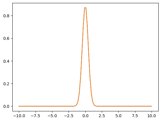
For our data that we provide to our neural network, we’ll give it the following initial condition (e.g. data at time t = 0):
\[u(x,t = 0) = \frac{1}{\sqrt{4\pi(0.1)}}\exp\left( - \frac{x^{2}}{4k(0.1)} \right)\]Which gives the following Initial condition:

Now we could use every point in time and space but that would require an infinite number of evaluations! Instead, we can sample points in space and time with these points being colloquially known as colocation points as well sample our initial condition/data points. This means for PINNs, we can use the standard mean square error for both our loss functions:
\[\mathcal{L}_{obj} = \mathcal{L}_{Residual} + \mathcal{L}_{data} = \frac{1}{n}\sum_{i}^{n}\left\lbrack R^{i}(x,t) \right\rbrack^{2} + \frac{1}{m}\sum_{j}^{m}\left( u_{net}^{j} - u_{data}^{j} \right)^{2}\]Where Ri is the residual of the neural network evaluated at some point i, unetj and udat**aj is the neural network and the ground truth at point j respectively.
Now you might be wondering why I chose this equation and initial condition. Well, it’s because this setup has an analytic solution that we can compare our results to. This is given as:
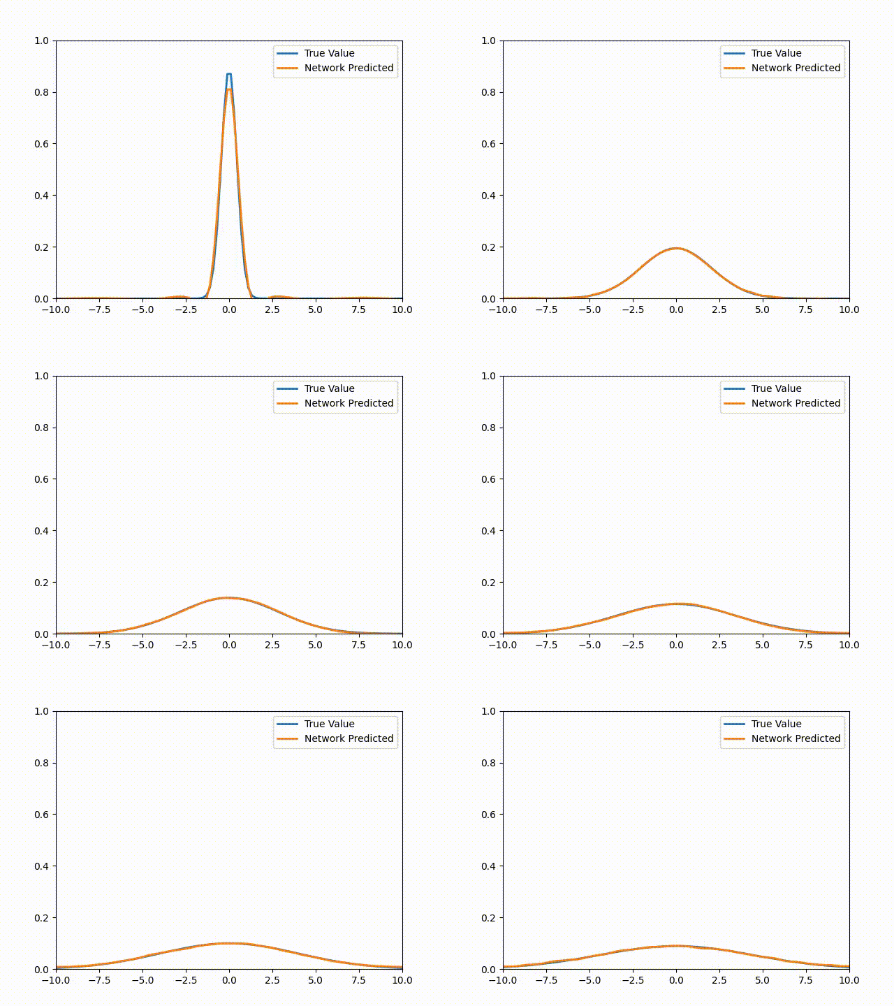
\[u(x,t) = \frac{1}{\sqrt{4\pi(t + 0.1)}}\exp\left( - \frac{x^{2}}{4k(t + 0.1)} \right)\]Setting t = 0 gets us to our initial condition. Note that for more complicated equations or geometries, there’s almost never an analytic solution (if there was then we wouldn’t be here talking about PINNs would we?). Once we train this PINN we get the following animation (The actual solution is included for comparison):

Pytorch Code
The coding tutorial is available in a Colab notebook here or at its GitHub repository. I’m going to use my own classes here to make things easier (Higher order gradients can get annoying to deal with in PyTorch this just makes it easier). You don’t need to understand the inner workings of this code just know that it wraps around the network so that when an input is given, the wrapped network returns not only the output but the desired derivatives. Theres also another example using the spring equation in the tutorial.
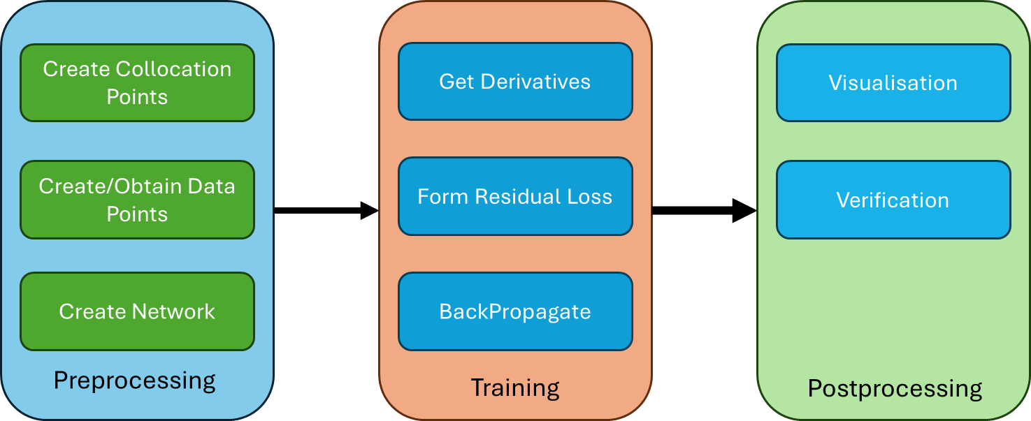
The following is a rough outline of how PINNs work:

Disadvantages of PINNs
While PINNs can seem like a silver bullet in the world of simulation, there are difficulties that need to be addressed. Just like in traditional simulations there ‘no free lunch’ – any advantages we gain with one method seemingly creates a problem elsewhere. PINNs are no different.
Validity of Results
From an FEA point of view the first issue is interpreting how reliable the results are. While in the above example we had an analytic solution, in practice we never have a 100% ground truth (In structural engineering we might have some hand calcs and small amount of data to double check). The simplicity of the PINN is the issue here – The residual and data losses are considered ‘soft losses’ can never be exactly satisfied. Furthermore, it is difficult to interpret the convergence of our results in that how do we know that the network has correctly converged on the right dynamics? With numerical methods such as FEA and CFD we have some mathematical guarantees as well as decades of empirical results to support our model.
Currently most PINN papers use traditional methods as their ground truth for how accurate there PINN dynamics are.
Training The Network
Perhaps the biggest difficulty currently is the actual training of the network itself to learn the equations. There are many issues surrounding this part but the mains points being:
Residual Loss topology
Balancing of loss terms
Network Architecture
Residual Loss Topology
The residual loss turns out to have a very ‘flat’ like landscape or topology. This can make it difficult to find the minimum with gradient descent. What this means for PINNs is that it can represent the incorrect dynamics. From a mathematical point of view this makes some sense as the solutions to differential equations are not unique unless appropriate boundary and initial conditions are applied. An example of this is, if you remember from high school calculus, integrating a function. Suppose we have the equation we want to solve:
\[\frac{dF(x)}{dx} = x\]Then using high school calculus to solve this we can simply integrate:
\[\int x\ dx = F(x) = \frac{x^{2}}{2} + C\]Unless we give some boundary condition for F(x), we have infinite solutions as C can be anything and still satisfy our initial differential equation! The other way to think about it is if in the case of physics: If I only give you the forces acting on something, there’s no way you can give me the velocity of that object. As such, this makes the residual loss function difficult to deal with as the neural network can satisfy the residual loss while not satisfying the data term.
Balancing the loss terms
Another difficulty is that the network can optimize one loss over the other which can lead to the wrong dynamics being produced. A given reason is that the magnitude of each loss relative to each other can be quite dramatic. As a result, one often introduces a weighting factor:
\[\mathcal{L}_{obj} = \mathcal{L}_{residual} + \lambda\mathcal{L}_{data}\]Where λ is the weighting factor. A large amount of research has gone into methods to automatically weight these loss terms, so they are similar in magnitude. The outline of different weighting strategies by NVIDIA gives a good summary of the different strategies (link).
Network Architecture
Finally, the size of the architecture of the network is still under research. Unlike image-based tasks (which typically use convolution-based networks) and language tasks (which use transformers), PINNs lack an effective network architecture. Many possible architectures are detailed here (link).
Complex Geometries and Boundaries
PINNs are often continuous in nature as opposed to the discrete representations in standard numerical methods. This presents a challenge for representing complex boundaries in PINNs with the current formulation and limits the domain to simple geometries like squares and rectangles. The continuous nature of PINNs makes it difficult to exactly define the boundary of the domain. One might say that a close enough is good enough, this won’t be true for chaotic systems such as turbulence where small perturbations of the geometry can create large changes.
Conclusion
This ends my introduction to PINNs. While PINNs have shown great promise, I do feel there is still a lot of progress that needs to be made before PINNs can become viable (Deep Learning community is overly optimistic on how well these networks can be used to solve real-world problems). There are also extensions to PINNs such as Deep O Nets and graph based PINNs (which work on meshes similar to many traditional methods)
If you want to know more about PINNs I recommend checking the following links (I am not affiliated with any of these parties):
