Operator Learning and Implementation in Pytorch
- What are Operators?
- Deep O Net Architecture
- Input Shape to Compute an entire Minibatch
- DeepOnet Data Driven Training
- Results
- Where to go from now?
Operator Networks are a type of neural network used in physics informed machine learning. Rather than learning a single solution or scenario to some PDE, operator networks try to learn the a family of solutions space. For example, instead of having a neural network learn the dynamics of a spring of specific stiffness k, an operator network would learn the solutions of the spring system for all (or at least within a specified range) of spring systems. There are a slew of different architectures and implementations for operators but in this post we’ll look into the Deep Operator Networks or Deep O’nets by Lu et al. We’ll look at the practical implications for deep O nets such as input shapes and sizes and other considerations.
The accompanying notebook can be found here
What are Operators?
Without going into too much maths, we can think of Operators as an object that takes in a function and spit out another function. A common example of an operator would be the derivative operator. We give the derivative operator an input function (say sin(x)) and it spits out another function (in this case cos(x)). Indefinite integration is also another example of an Operator. To express say indefinite integration we define a mapping G that takes in a function u(x) and outputs another function G(u)(x):
\[G\left(u\right)\left(x\right)=s_0+\int_{0}^{x}{u\left(t\right)\ dt}\]Where s0 is the integration constant. The formulation of operators is very general and so what they can take in and spit out can be very general (for example they can also be autoregressive, taking in some state i and spitting out the next stat i+1). Just keep in mind that operator networks are designed to provide a family of solutions rather than a solution to a single instance. So, in the case of integration, we want our Operator network to be able to integrate over a range of different functions (such as cos, sin, exp, polynomials etc) not just a single function.
The formulation of operator learning is very similar to other Deep learning tasks such as generative tasks such as art and natural language processing where we give the network a function (in the form of a prompt) and it spits out another function which is some image or text respectively.
Deep O Net Architecture
Deep O Nets by Lu et al. learns a mapping G from an input function u to and output function G(u). We can then also query values of G(u) for points y. All in all, we aim to train a network G that takes in the inputs: a function u, and querying points y to learn the G(u)(y)
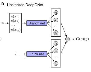
The basic network is straightforward. It comprises of 2 sub networks: the branch network and the trunk network. We will just use a simple MLP for both the trunk and branch networks. This comes from the ‘Unstacked’ DeepOnet from the paper:

The branch network takes in as input the function u(x) and maps it to some latent vector b. The trunk network takes in the ‘querying’ points (point we want to sample G(u)) and maps it to some latent vector t. we then perform element wise multiplication and sum the results to get our output G(u)(y). The element wise multiplication implies that the latent states t and b must be of the same shape/broadcastable (more on that later). In my implementation, I replace the final summation with an additional linear layer. This makes the network more generalisable if the output function is multivariable.
We also need to discretize the function u at different locations xi so we input it to the branch net:
\[u\left(x\right)\rightarrow\left[u\left(x_1\right),u\left(x_2\right),\ldots,u\left(x_n\right)\right]\]This introduces two considerations/hyperparamters: the number samples/sensors for u as well as the domain of x. It is implicitly implied that the sensor location (xi) is fixed for all functions u and that the domain of u is the same for all functions (e.g. for all u(x), x ∈ [0,1]). Fortunately, we can often rescale our functions to fit inside the fixed domain, perform the operation, and then reverse the scaling to get back to our original function.
Input Shape to Compute an entire Minibatch
An important thing to note is that the number of points y we choose to sample is independent of the number of sensors we use to discretize u. This means If we want to do everything in a single forward pass for each minibatch, we need two “batch” dimensions: one for the number of input functions and one for the number of points we are sampling for each input function. Thankfully using broadcast rules and how pytorch’s nn.Linear class works (which looks at the last dimension size as input) we can compute the entire minibatch a single forward pass for an arbitrary number of input functions and sampling points. We ensure our tensors have the following shapes:
Table 1 General Shape and dimension for each element in a minibatch
| Variable | Shape |
|---|---|
| u input | [B,1,M] |
| y input | [B,N,D] |
| G(u)(y) output | [B,N,O] |
Let’s break this down.
B is the size of the batch dimension and represents the number of u functions are in our mini batch (in this case 1000).
The 2nd dimension of u is set to always set to 1. This ensures that the output shape of the branch net will match the output shape of the trunk net.
M is number of sensors/input size to the branch net (in this case 100).
N is the number of point y we are querying (in this case 100)
D is the input size of the trunk net (in this case 1)
O is the output size of the entire DeepONet ( in this case 1)
Note that when u and y are passed through the branch and trunk net respectively, the latent features b is of shape (B,1,L) and t is of shape (B,N,L), where L is the dimension size of the latent space allowing for element wise multiplication. Using broadcasting, we ensure that within a single batch, each b vector of size L is applied to the N different t vectors which represent the t vectors from each sampled y point.
DeepOnet Data Driven Training
We’ll use a similar example to the first example outlined in the paper of solving a 1D ODE system for a purely data driven approach:
\[\frac{d}{dx}F(x) = u(x)\\,\\x \in \lbrack 0,2\rbrack\] \[F\left(0\right)=0\\]The mapping G for an input function u(x) for a point y is:
\[G\left(u\right)\left(y\right)=\int_{0}^{x}{u\left(t\right)\ dt}\] \[G\left(u\right)\left(0\right)=F\left(0\right)=0\ \ for\ all\ u\]We generate a dataset of 10,000 random u(x) functions. Each function u(x) is uniformly discretized to 100 points between 0 and 2. Furthermore, for each function u(x), we also randomly sample 100 points along the domain. These represent out y or query points.
In this case we use Chebyshev polynomials to generate the random functions. It doesn’t really matter the method of generating the random functions ( in the paper they also use Gaussian random fields to generate the functions). We can then integrate each u(x) to get the data of G(u)(y). This results in 10000x100 = 1,000,000 data points for our example.
For the data driven approach when we put this into a dataloader, we get a batch of triplets: (u, y, G(u)(y)). Using a minibatch of 1000 each variable then has the following shape. Feel free to modify the parameters as you wish!
Table 2 Shape and Dimensions for each minibatch
| Variable | Shape |
|---|---|
| U | [1000,1,100] |
| Y | [1000,100,1] |
| G(u)(y) | [1000,100,1] |
Our training model has the following setup:
| Epochs | 7500 |
|---|---|
| Minibatch | 1000 |
| Initial Learning Rate | 5e-4 |
| Learning Rate Schedular | StepLR(gamma = 0.95,step_size = 1000) |
| Optimiser | Adam |
| Input Features | Hidden Features | Depth | Output Features | |
|---|---|---|---|---|
| Branch Net | 100 | 75 | 4 | 75 |
| Trunk Net | 1 | 75 | 4 | 75 |
| Final Linear Layer | 75 | - | 1 | 1 |
For validation, we track the accuracy of our deep O net on the following function
\[u\left(x\right)=\sin{\left(ax\right)}\]Which has the following indefinite integral (note F(0) = 0)
\[F(x) = \int_{0}^{x}{\sin(at)\ dt} = \frac{1}{a}(1 - \cos{(at)})\\\]Results


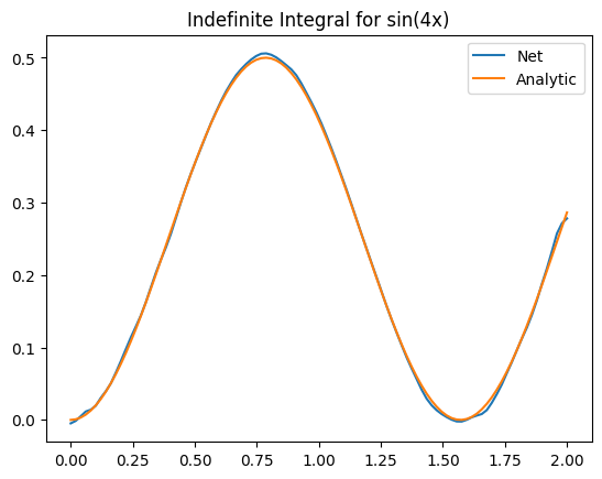
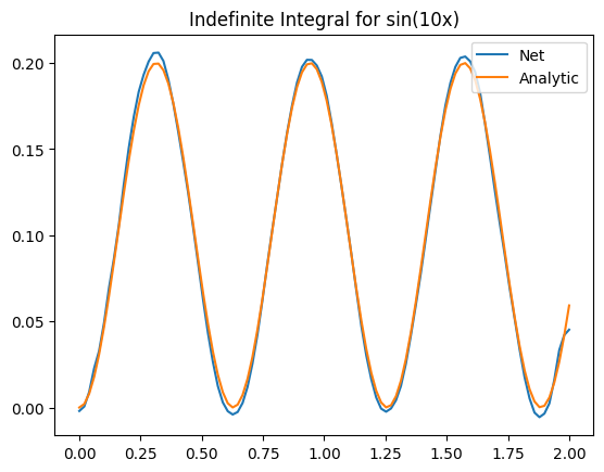
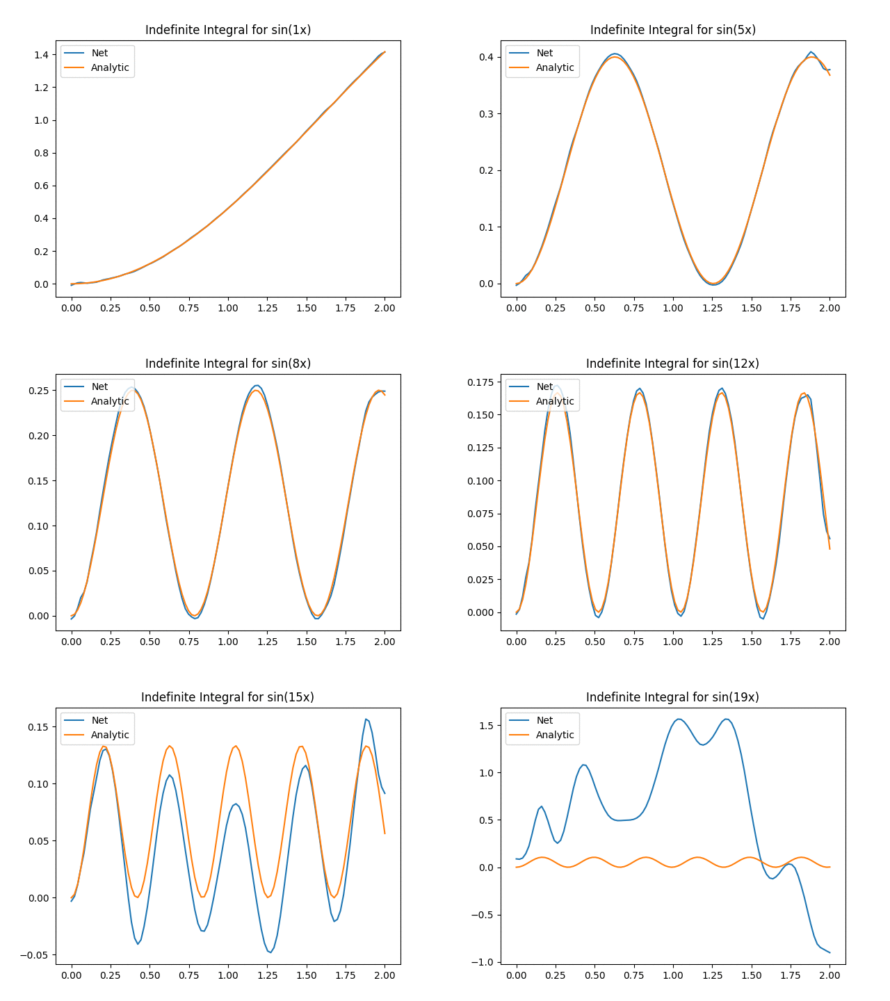
Not bad aye? One thing to keep in mind is that we now have to start worrying about inputting functions that are too far off our original training distribution. This is the extrapolation problem and the exact same problem as giving new images to networks. In our case we can see the effect when we start increasing the value of a in the above function:

We can see that for a > 14, the Onet starts struggling. There could be a myriad of reasons (e.g. not training enough, out of distribution etc) but the key part here is an important part about deep learning in general we need to think about: We have to verify and validate our results! While neural networks are powerful tools, they have their limitations and aren’t always the silver bullet that will solve all our problems!
Where to go from now?
This is a very simple example of training an Operator network but isn’t useful other than for demonstration (I mean how to get the data I literally had to use an existing method of numerical integration!) There are two paths from here.
The first is to improve the predictive capabilities of the Operator networks. Just like resnet for images or transformers for NLP, operator networks can significantly improve their performance depending on the network you use. In our example we just used a simple MLP for our branch and trunk networks. The current state of the art are Fourier Neural Operators (FNOs) and its adaptive counterpart which you can read about here and here.
The second is reducing the reliance on data. Here we had plenty of data to draw from as well as dense number of sensors. However, as we go to higher dimensions or real life, the number of sensors and data available decreases. For example, we might only have thermal data but we want to analyse air flow. In this scenario, we can borrow ideas from physics informed neural networks (PINNs) to fill in the blanks for us. PINN based learning also help us better steer the Onet to solutions that obey physical laws at the cost of increased computational resources. The accompanying notebook has an example of using the PINN approach to solve the above problem without the need for data.
